I just read Clocking the mind: mental chronometry and individual differences by Arthur R Jensen (2006). It is a wonderful tome of information that belongs in the same category as Response times by R Duncan Luce (1986) and Reaction times edited by WT Welford (1980). All three of these books delve into the use of mental chronometry (i.e. reaction times) in psychology. The books by Luce and Welford focus on cognitive psychology, whereas Jensen reviews mostly differential psychology. Clocking the mind, however, is still a great resource for cognitive psychologists as Jensen reviews a plethora of factors that are vital for any experiment measuring reaction time.
Below are my favourite excerpts from the book.
Simple and choice reaction time
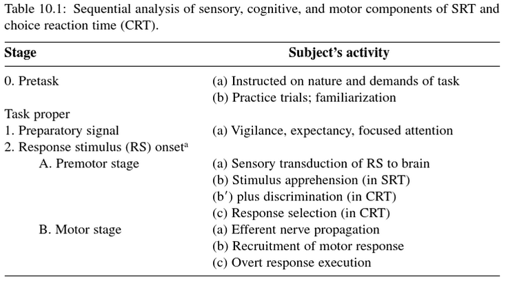
I’m a sucker for tables that detail the processes that compose reaction time. Below is Jensen’s interpretation. (I’ve previously posted about the interpretations by R Duncan Luce and FC Donders.)
The split-half reliability coefficients based on odd-even trials are high (around .90 with as few as 30 trials) for both RTm and MTm, and test-retest reliability for 15 trials measured on each of two days is about .80 for RTm and MTm… Several practice trials followed by 60 test trials are typically required for simple RT to attain a reliability coefficient of about .90.
As CRT tasks increase in information processing demands, there is a regular decrease in the correlation between CRT and SRT. SRT and 2-choice RT have about 80% of their true-score variance in common; SRT and 8-choice RT have only about 50% in common (Jensen, 1987a, p. 139).
In groups of college students, for example, there is an average difference of 40-50 ms even between SRT and two-CRT, when there is an optimal preparatory signal and the RT in each case is simply a bright green light going “on,” always in the same location (SRT), or randomly in one of two locations (CRT)… It is also important to note that the effect of increasing task complexity is to increase the slower RTs much more than the faster RTs.
…RT and MT. These measures are relatively independent, correlating with each other only about .30… It appears that CRT reflects mostly information processing whereas MT reflects mostly sensorimotor ability.
Masking the reaction stimulus
To make it difficult or impossible for participants to leave the home key before completely processing the precise location of the response stimulus, some researchers have all the lights go “on” the instant the participants release the home key, in order to lessen the possibility for participants to leave the home key prematurely and continue processing the location of the response stimulus while in transit (Smith & Correau 1987). This “masking” of the reaction stimulus at the instant of participants response is intended to discourage response strategies that interfere with conformity to Hick’s law.
Skewness
A simple but crude measure of skewness is Sk = 3(Mean – Median)/SD. A more precise and the preferred measure, included in most computerized statistical packages, is R. A. Fisher’s g1 = Σ(X – Xbar)3/N(SD)3.
Kurtosis, or the degree of peakedness (or flatness) of a distribution is measured by Fisher’s g2 statistic: g2 = [Σ(X – Xbar)4/N(SD)4] – 3.
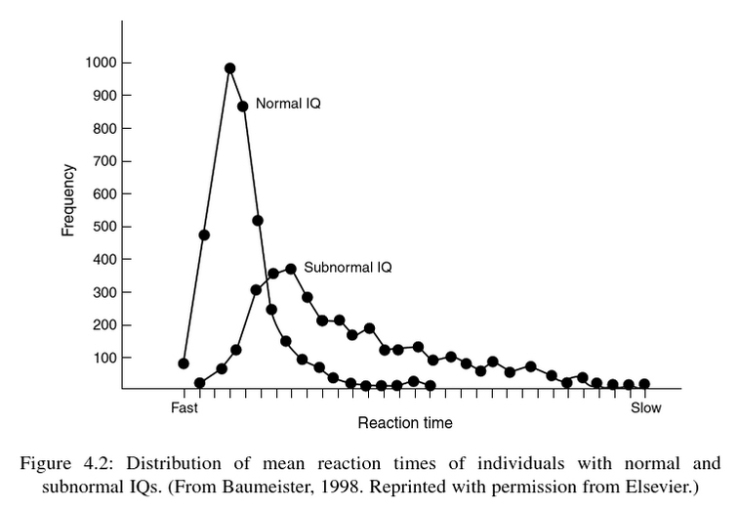
The total distribution of a given individual’s RTs over n trials is not symmetrical but is necessarily skewed to the right (i.e., longer RT), because there is a lower physiological limit of RT and there is no naturally imposed upper limit of RT.
RT vs. RTSD
Also, the RT and RTSD behave quite differently in too many ways to make it seem likely that they are totally non-independent variables. In the Hick paradigm, for example, whereas RTm (or RTmd) shows a perfectly linear relationship to bits, or the binary logarithm of the number of RS alternative, RTSD shows a perfectly linear relationship to the number of alternatives per se and is exponentially related to bits.
Trials before and after errors
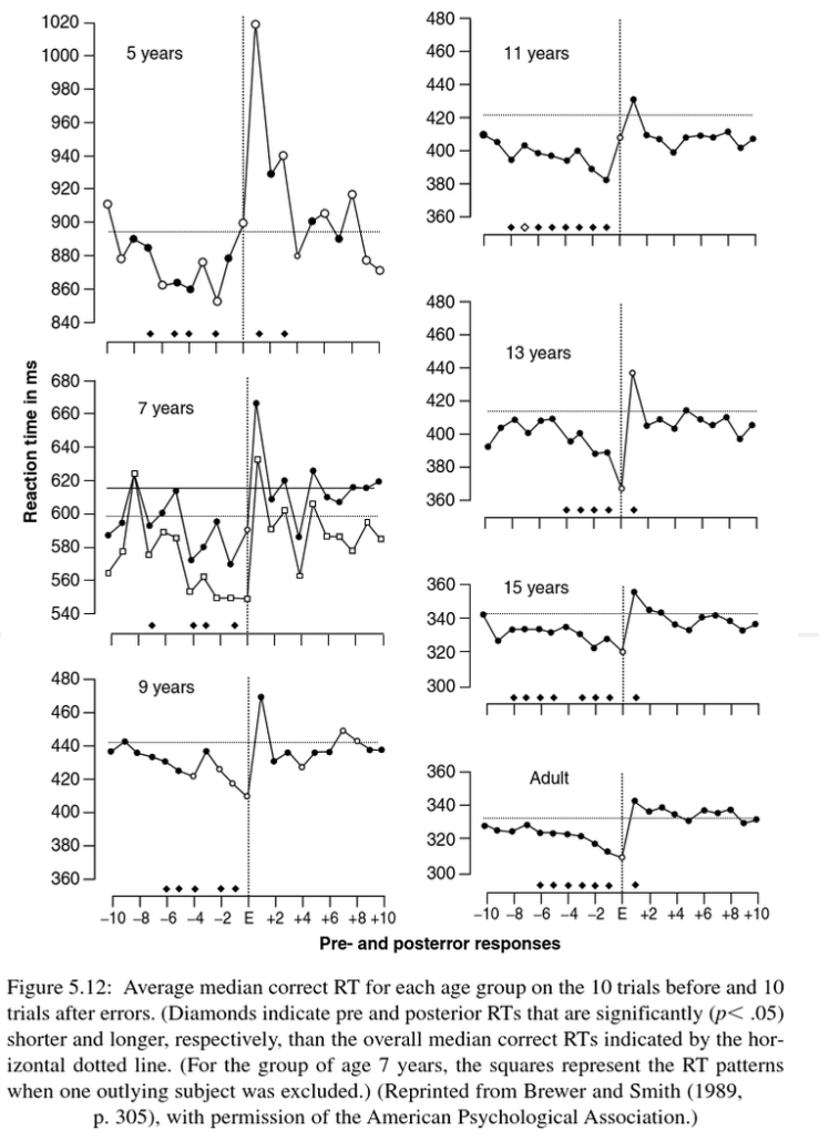
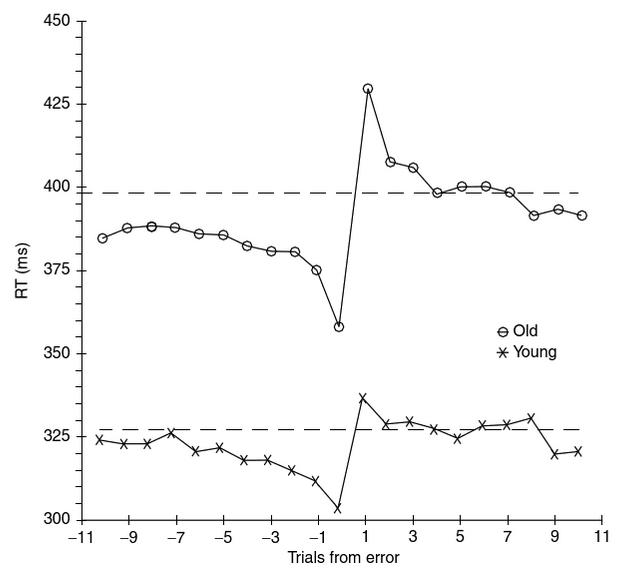
But the most interesting finding in this study is the nature of the RTs on the trials preceding and following an error response, which tend to average out in a subject’s mean RT based on many trials. Figure 5.12 shows the mean RTs of the 10 trials preceding and the 10 trials following an error response in each age group. At every age, subjects appear to be continually testing themselves for the fastest response speed they can get away with without risking an error, and when an error occurs they immediately go back to a more cautious speed of responding. The RTs for 5- and 7-year olds are markedly more erratic and the posterior effects of an error are much greater than in the older groups, indicating a less “fine-tuned” control of RT. Note also that it takes longer for the younger groups to recover to a faster RT after an error response; slower than average RTs occur for several trials following the error… Old adults resemble the 13 year-olds (Figure 6.13).
I’ll upload a better version of the first figure when I’m back in the lab.
Effects of practice
SRT to light, with maximum S-R compatibility shows virtually no practice effect (i.e., improvement) in RT after the first 10 trials. For CRTs, however, the practice effect persists over at least 10,000 trials and the CRT is a decreasing linear function of the logarithm (log10) of the number (N) of trials. The average slopes of the regression of CRT on log10N for 2-, 4-, and 8-choice RTs derived from a number of studies were -0.099, -0.169, and -0.217 s (Teichnet & Krebs, 1974, p. 82)… On a 2-choice RT task, for example, if the RT on the first trial is 0.725 s, it is 0.626 s on the 10th trial, 0.527 s on the 100th trial, and 0.428 on the 1000th trial… The investigator takes advantage of the fact that the largest practice effects occur in the early trials, and allows a fair number of discountable practice trials (e.g., 20 or so) before beginning the test trials.


