Confidence intervals in within-participant design: a tutorial on the Cousineau-Morey method

A few years ago I wrote about the problem with typical confidence intervals in within-participant designs (also called repeated measures designs). “The problem with confidence intervals is that they are calculated based on the between-participant and within-participant variances. The ANOVA significance tests, however, are based on only the within-participant variance. The between-participant difference is subtracted to improve the power for testing within-participant effects. Thus, the confidence intervals overestimate the error terms in the ANOVA and prevent us from using a rule of eye to determine statistical significance.”

There are two popular ways to remove the between-participant variance from the confidence intervals. Let’s refer to these normalised intervals as within-participant confidence intervals. The two methods are the Cousineau-Morey method and the Loftus-Masson method. Today, we will focus on the Cousineau–Morey method, which has three advantages over the other method.

1. On average, a 95% confidence interval will include 83% of replication means (5 out of 6; Cumming and Maillardet 2006)
2. The confidence intervals can be calculated before running a repeated measures ANOVA
3. A unique error bar is calculated for each mean

Let’s talk about calculating confidence intervals. The formula for typical confidence intervals (that include between- and within-participant variance) is:

CI = Mean +/- t(1-alpha/2, n-1) * SD / sqrt(n)

A few notes:

• SD is the standard deviation
• n is the number of participants
  • SD / sqrt(n) is the standard error
• the t-value for an alpha of .05 approaches 1.96 as n approaches infinity

Let’s calculate typical 95% confidence intervals for some sample data. Below are reaction times from a 2×2 repeated measures design with 18 participants.

Number	A1	A2	B1	B2	Participant mean
1	241	178	253	215	221.75
2	209	236	306	344	273.75
3	211	170	462	521	341.00
4	167	155	204	204	182.50
5	190	166	225	271	213.00
6	207	189	276	281	238.25
7	163	157	231	266	204.25
8	172	149	284	251	214.00
9	171	174	199	263	201.75
10	187	196	196	207	196.50
11	181	204	192	244	205.25
12	164	171	250	268	213.25
13	139	139	181	191	162.50
14	153	138	175	198	166.00
15	165	169	209	245	197.00
16	158	174	204	229	191.25
17	199	207	294	292	248.00
18	180	188	215	262	211.25
Mean	180.9444	175.5556	242.0000	264.0000	215.6250
SD	25.1173	24.9946	67.7782	74.6309	41.1938

Calculate a 95% confidence interval for the grand mean

We start with the formula from above:

• CI = Mean +/- t(1-alpha/2, n-1) * SD / sqrt(n)
• 95% CI = 215.6250 +/- t(1-.05/2, 18-1) * 41.1938 / sqrt(18)
• 95% CI = 215.6250 +/- t(.975, 17) * 41.1938 / 4.2426
• 95% CI = 215.6250 +/- 2.1098 * 9.7096
• 95% CI = 215.6250 +/- 20.4853

Therefore, the 95% confidence interval of the grand mean is [195, 236]. One important note, you can’t normalise the confidence interval for the grand mean.

Calculate the typical 95% confidence intervals for the four conditions

The conditions in the 2×2 experiment are simply labeled A1, A2, B1, and B2. These typical confidence intervals will include the between- and within-participant variance. Use the same formula as above and you should get the following confidence intervals:

• A1 [168, 193]
• A2 [163, 188]
• B1 [208, 276]
• B2 [227, 301]

A graph of the means and 95% confidence intervals is below. We will see how much these typical confidence intervals shrink when we exclude the between-participant variance.

If this were a between-participant design, then these confidence intervals and the rule of eye tell us that there will be a significant difference between A and B. It is hard to say whether A1 is different than A2 and whether B1 is different than B2. Let’s see how this changes when we normalise the confidence intervals.

Calculate the within-participant 95% confidence intervals for the four conditions

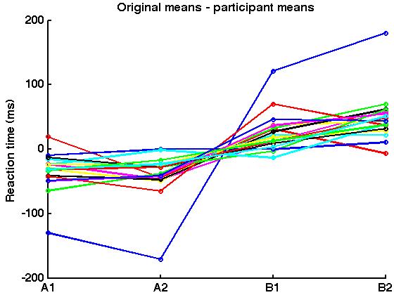
Now the fun begins. Before we do any normalisation, let’s take a look at all the data from the 18 participants. Below is a figure of the means in the four conditions (A1, A2, B1, B2) for each participant. Notice that some participant have shorter or longer reaction times than others. This is between-participant variance, and we are going to remove it to calculate the within-participant confidence intervals.

We can remove the between-participant variance with one simple step. Simply subtract each participant’s mean (the last column in the table above) from each of the four conditions (A1, A2, B1, B2). This will balance each participant’s data around 0 ms. Take a look at the results below.

We have now removed the between-participant variance and we could go ahead with calculating within-participant confidence intervals. However, these reaction times no longer make sense. To make the data appropriate for the conditions, simply add the grand mean (215.6250 ms, also in the table above) to all the normalised means. This is shown in the following figure.

Notice that the patterns in the last two figures are the same, but the reaction times are now in a normal range for the conditions (i.e. we have removed the between-participant variance, but the normalised means are the same as the original means).

There is one other issue to discuss that is specific to these data. Compare the variability in the four conditions in the first line graph (the original data) to the third line graph (the normalised data). The variability between most participants in the normalised data is smaller, except for the weird data from one participant who has shorter normalised RTs for A1 and A2 and longer RTs for B1 and B2. (The original data shows that the participant had RTs that were longer in only B1 and B2; however, normalising the data made the data abnormal in all the conditions.) We usually see less variability for normalised data but that is not always the case. The weird data is going to make the 95% within-participant confidence intervals larger in A1 and A2 than the typical 95% confidence intervals.

Fun statistical fact, if you run a 2×2 repeated measures ANOVA on the original data and then the normalised data, you will get the same results for the two main effects and the interaction (the within-participant effects). Remember that normalising the data removes the between-participant variance, which is also removed by a repeated measures ANOVA. By normalising the data, we have removed the between-participant variance for the ANOVA. Now, there is one difference in the ANOVA on the normalised data. If you look at the between-participant effects, you will notice that there is no F value. The F value cannot be calculated because the error term is zero – there is no between-participant variance because we removed it!

We can now calculate within-participant confidence intervals, but we need to make one change to the original formula (this is the Morey part of the Cousineau-Morey method).

CI = Mean +/- t(1-alpha/2, n-1) * SD / sqrt(n) * sqrt(c / (c-1))

The addition is sqrt(c / (c-1)), where c is the number of within-participant conditions. In our 2×2 example, there are four conditions. Evaluating sqrt(4 / (4-1)) gives us 1.15, so this correction factor is going to make the confidence intervals slightly larger. Note that the largest increase in the confidence intervals would be with 2 within-participant conditions [sqrt(2 / (2-1)) = 1.41] and that this correction decreases with more conditions.

The confidence intervals need to be made slightly larger because normalising the data introduced positive correlation among the data, and this decreases the standard deviation of the data. This bias is countered by the correction factor.

Let’s calculate the 95% confidence intervals for the normalised data using the CI formula with the correction factor.

• CI = Mean +/- t(1-alpha/2, n-1) * (SD / sqrt(n)) * sqrt(c / (c-1))
• 95% CI = Mean +/- t(1-.05/2, 18-1) * (SD / sqrt(18)) * sqrt(4 / (4-1))
• 95% CI = Mean +/- t(.975, 17) * (SD / sqrt(18)) * sqrt(4/3)
• 95% CI = Mean +/- 2.11 * (SD / 4.24) * 1.15

The normalised means and standard deviations are as follows.

• A1 M = 180.9444, SD = 30.0029
• A2 M = 175.5556, SD = 36.5616
• B1 M = 242.0000, SD = 30.8476
• B2 M = 264.0000, SD = 37.9874

Which gives us the following 95% within-participant confidence intervals.

• A1 [164, 198]
• A2 [155, 197]
• B1 [224, 260]
• B2 [242, 286]

Below is a graph of the means and these within-participant 95% confidence intervals. Compare the size of the confidence intervals to the typical 95% confidence intervals in the first graph.

The confidence intervals in B1 and B2 are smaller than the typical 95% confidence intervals. As we noted earlier, the 95% within-participant confidence intervals in A1 and A2 are actually larger because of weird data from one participant.

Calculate the 95% within-participant confidence intervals for A vs. B

We just calculated confidence intervals for the four conditions, which assumes that there was a significant 2×2 interaction. There could be, however, just a main effect of A (A1, A2) vs. B (B1, B2). In this case, we would calculate confidence intervals for just A and B. The process is very similar but you begin by calculating the mean of A1 and A2 to get A and B1 and B2 to get B for each participant. Now that you have A and B, you can normalise the data and then calculate the 95% within-participant confidence intervals. The number of conditions is now two (A and B), so sqrt(c / (c-1)) = sqrt(2/1). The confidence intervals should work out to be as follows:

• A [156, 200]
• B [231, 275]

Calculate the 95% within-participant confidence interval for the grand mean

Let’s assume that the 2×2 ANOVA had no significant main effects or interactions. We would probably want to report the grand mean (for all conditions combined) and the appropriate 95% confidence interval. Can we calculate a 95% within-participant confidence interval for the grand mean? The short answer is “no,” but let’s give it a try.

We start be finding the mean of the four conditions for each participant. Now, subtract each participant’s mean from this mean. The problem is that these means are one and the same! The normalised data would end up being the grand mean for each participant (hence, no variability). Therefore, if you want to calculate a confidence interval for the grand mean, you need to calculate a typical confidence interval. This was the first confidence interval that we calculated, and it was [195, 236].

Future topics

If you want to dig deeper into this topic, then I recommend Baguley (2012) and Cousineau and O’Brian (2014). Perhaps someday I will give a tutorial on the Loftus-Masson method. I remember reading somewhere about how to use these methods with mixed designs (that have within- and between-participant factors). If I ever figure that out, I’ll post about it.